TabR
Published:
This article introduces the TabR model, a retrieval-augmented model designed for tabular data. It is part of a series on tabular deep learning using the Mambular library, which started with an introduction to using an MLP for these tasks.
Architecture Overview
TabR is a retrieval-augmented tabular deep learning method that leverages context from rest of the dataset/database to enrich the representation of the target object, producing more accurate and up-to-date responses. It uses related data points to enhance the prediction. The TabR model consists of three main components: the encoder module, the retrieval module, and the predictor module. The architecture of the TabR model is illustrated in the figure below:
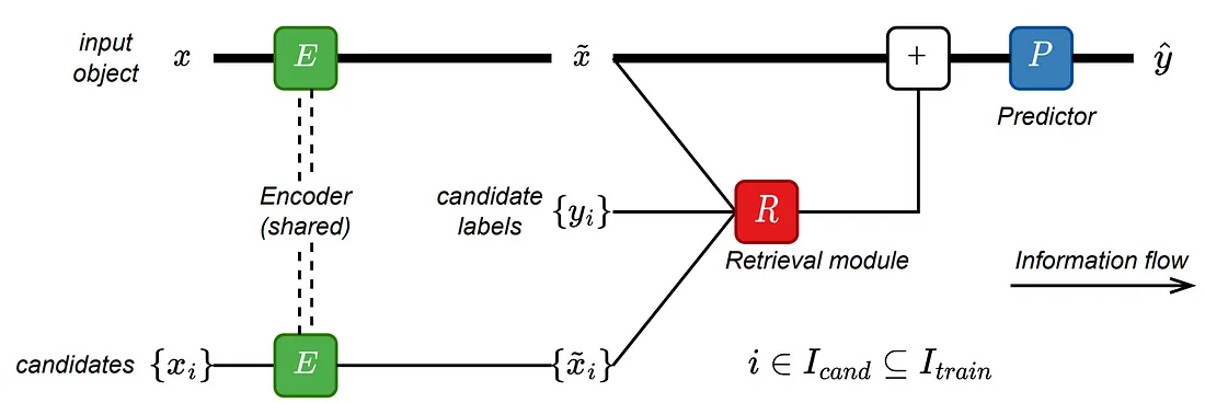
The model is a feed-forward network with a retrieval component located in the residual branch. First, a target object and its candidates for retrieval are encoded with the same encoder E. Then, the retrieval module R enriches the target object’s representation by retrieving and processing relevant objects from the candidates. Finally, predictor P makes a prediction. The bold path highlights the structure of the feed-forward retrieval-free model before the addition of the retrieval module R.
Model Fitting
Now that we have outlined the TabR model, let’s move on to model fitting. The dataset and packages are publicly available, so everything can be copied and run locally or in a Google Colab notebook, provided the necessary packages are installed. We will start by installing the mambular package, loading the dataset, and fitting TabR. Subsequently, we will compare these results with those obtained in earlier articles of this series.
Install Mambular
pip install mambular
pip install delu
pip install faiss-cpu # faiss-gpu for gpu
Prepare the Data
from sklearn.datasets import fetch_california_housing
from sklearn.model_selection import train_test_split
from sklearn.metrics import mean_squared_error
from sklearn.preprocessing import StandardScaler
# Load California Housing dataset
data = fetch_california_housing(as_frame=True)
X, y = data.data, data.target
# Drop NAs
X = X.dropna()
y = y[X.index]
# Standard normalize features and target
y = StandardScaler().fit_transform(y.values.reshape(-1, 1)).ravel()
# Train-test-validation split
X_train, X_temp, y_train, y_temp = train_test_split(
    X, y, test_size=0.5, random_state=42
)
X_val, X_test, y_val, y_test = train_test_split(
    X_temp, y_temp, test_size=0.5, random_state=42
)
Train TabR with Mambular
from mambular.models import TabRRegressor
model = TabRRegressor()
model.fit(X_train, y_train, max_epochs=200)
preds = model.predict(X_test)
model.evaluate(X_test, y_test)
Mean Squared Error on Test Set: 0.1877
Compared to MLP-PLR and MLP-PLE, it is a comparable performance. However, compared to XGBoost, it is not a good fit. Let’s try the TabR with PLE as numerical pre-processing as already used in the FT Transformer article.
model = TabRRegressor(
                  numerical_preprocessing='ple'
                  )
model.fit(X_train, y_train, max_epochs=200)
preds = model.predict(X_test)
model.evaluate(X_test, y_test)
Mean Squared Error on Test Set: 0.18666
Compared to XGBoost, this approach does not seem to be a good fit. Let’s try TabR with PLR embedding as already used in the MLP article.
model = TabRRegressor(use_embeddings=True,
                  embedding_type='plr',
                  numerical_preprocessing='standardization'
                  )
model.fit(X_train, y_train, max_epochs=200)
preds = model.predict(X_test)
model.evaluate(X_test, y_test)
Mean Squared Error on Test Set: 0.1877
Again, compared to XGBoost, this approach does not seem to be a good fit. Therefore, let’s try with an alternative numerical preprocessing method — let’s try MinMax scaling.
model = TabRRegressor(use_embeddings=True,
                  embedding_type='plr',
                  numerical_preprocessing='minmax'
                  )
model.fit(X_train, y_train, max_epochs=200)
preds = model.predict(X_test)
result=model.evaluate(X_test, y_test)
Mean Squared Error on Test Set: 0.1573
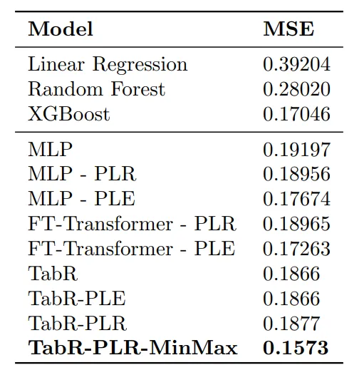
The Mean Squared Error (MSE) on the test set is 0.1573, making this our best-performing approach to date, even outperforming deep learning models as well as, tree-based methods like XGBoost.
Below we have summarized the results from all articles so far. Try playing around with some more parameters and improve performance even more. Throughout this series, we will add the results of each introduced method to this table: