
Chapter 5 (Notes)
Published:
5.2.2. Regression Metrics
- Regression refers to a predictive modeling problem that involves predicting a continuous (numeric) value rather than a class label.
- It is fundamentally different from classification tasks, which involve discrete labels or categories.
- Regression models are common in real-world tasks such as:
- Estimating prices (houses, cars, electronics)
- Predicting drug dosages based on patient characteristics
- Forecasting transportation demand
- Predicting sales trends using historical and market data
- Unlike classification, where accuracy can directly evaluate performance, regression requires error-based metrics.
- These metrics provide an error score summarizing how close the model’s predictions are to the actual values.
- Understanding and interpreting these scores is crucial for developing robust and interpretable regression models.
- There are four error metrics that are commonly used for evaluating and reporting the performance of a regression model; they are:
- Mean Squared Error (MSE).
- Root Mean Squared Error (RMSE).
- Mean Absolute Error (MAE)
- R-squared $(R^2)$
Mean Squared Error (MSE)
- Mean Squared Error (MSE) is one of the most widely used metrics for evaluating the performance of regression models.
- It measures the average of the squares of the errors—that is, the average squared difference between the actual and predicted values.
- MSE is a loss function used in least squares regression and also serves as a performance metric.
- It is the basis for least squares optimization, the core of many regression algorithms (e.g., Linear Regression).
- Highlights large errors, making it ideal when penalizing significant mistakes is important.

- Formula:
- Where:
- $n$ : Total number of data points
- $y_i$ : Actual (true) value of the $i^{th}$ data point
- $\hat{y}_i$ : Predicted value of the $i^{th}$ data point
- Characteristics:
- Always non-negative (since errors are squared).
- Units: Squared units of the target variable, making it less interpretable in its raw form.
- Sensitive to outliers: Squaring errors disproportionately penalizes large mistakes.
- Interpretation: Lower MSE values indicate better model performance.
- Use MSE when?
- You want to penalize larger errors more heavily.
- You’re optimizing with algorithms that rely on gradient descent.
- You are more interested in the overall performance than interpretability.
Root Mean Squared Error (RMSE)
- RMSE is the square root of the Mean Squared Error (MSE).
- It provides a measure of the average magnitude of the prediction error, but unlike MSE, it is in the same unit as the original data.
- RMSE gives a higher weight to large errors due to the squaring step in MSE.
- Formula
- Where:
- $n$ : Total number of data points
- $y_i$ : Actual (true) value of the $i^{th}$ data point
- $\hat{y}_i$ : Predicted value of the $i^{th}$ data point
- Here, squaring handles the magnitude, and the square root brings the unit back to original scale.
- It is more interpretable than MSE because it’s in the same scale as the target.
- It penalizes larger errors more heavily (like MSE).
- Here, Lower RMSE indicates better model performance.
Mean Absolute Error (MAE)
- MAE calculates the average absolute difference between predicted and actual values.
- It is a linear score, meaning all errors are weighted equally in proportion to their size.
- Formula
- Where:
- $n$ : Total number of data points
- $y_i$ : Actual (true) value of the $i^{th}$ data point
- $\hat{y}_i$ : Predicted value of the $i^{th}$ data point
$ y_i - \hat{y}_i $ : Absolute difference (always non-negative)
- Easy to interpret and in the same unit as the original target.
- Less sensitive to outliers than RMSE or MSE.
- Good for general error analysis, especially when large errors aren’t critical.
R-squared (Coefficient of Determination)
- R-squared $(R^2)$ measures the proportion of the variance in the dependent variable that is explained by the independent variables in the model.
- In simpler terms, it tells us how well the model fits the data.
- Formula
- Where,
- $y_i$ : Actual (true) value of the $i^{th}$ data point
- $\hat{y}_i$ : Predicted value of the $i^{th}$ data point
- $\bar{y}$: Mean of actual values
- Numerator: Sum of squared errors (residual sum of squares, RSS)
- Denominator: Total sum of squares (TSS)
Here,
R-squared Value Interpretation 1 Perfect prediction (all variance explained) 0 Model does not explain any variability < 0 Model performs worse than a horizontal line - A higher R-squared generally means a better fit, but not always.
- R-squared doesn’t indicate causality, and a high value may still be misleading if the model is overfitting or improperly specified.
- It is a relative measure, it **compares model vs baseline (mean)
5.3. Model Validation Techniques
- Model validation is the process of assessing how well a machine learning (ML) or artificial intelligence (AI) model performs — especially on unseen (new) data.
- It ensures that the model:
- Achieves its design objectives
- Produces accurate and trustworthy predictions
- Generalizes well beyond the training data
- Complies with regulatory and quality standards
- Purpose:
- Evaluate Model Performance: Confirms that the model works not just on training data, but on real-world, unseen datasets.
- Support Model Selection: Helps compare multiple models, choose the most appropriate one, and select optimal hyperparameters.
- Prevent Overfitting: Assesses the risk of overfitting by observing how model performance changes on validation vs training data.
- Build Trust: Ensures transparency and reliability, especially if validated by third-party or independent teams.
- Comply with ML Governance: Contributes to AI governance by enforcing policies, monitoring model activity, and validating data/tooling quality.
- Benefits:
- Ensures Generalization
- Guides Model Selection
- Improves Accuracy and Robustness
- Builds Regulatory Confidence
- Prevents Future Failures
- Without model validation, we risk deploying models that look good on paper but fail in practice.
5.3.1. Train-Test Split
- The train-test split is the most basic method of model validation.
- It involves splitting the dataset into two parts:
- Training set: Used to train the model
- Test set: Used to evaluate model performance on unseen data
- Common ratios include:
- 70% training / 30% testing
- 80% training / 20% testing
- 60% training / 40% testing (for very small datasets)
- Advantages:
- Simple and fast
- Good for large datasets
- Helps quickly estimate model performance
- Disadvantages
- High variance: Model evaluation may vary significantly based on how the data was split
- Risk of under- or over-estimating model performance due to random splits
- Not ideal for small datasets
5.3.2. Cross Validation
- Cross-validation is a more robust model validation technique where the model is trained and tested multiple times on different data subsets.
- Helps to assess how the model generalizes to an independent dataset.
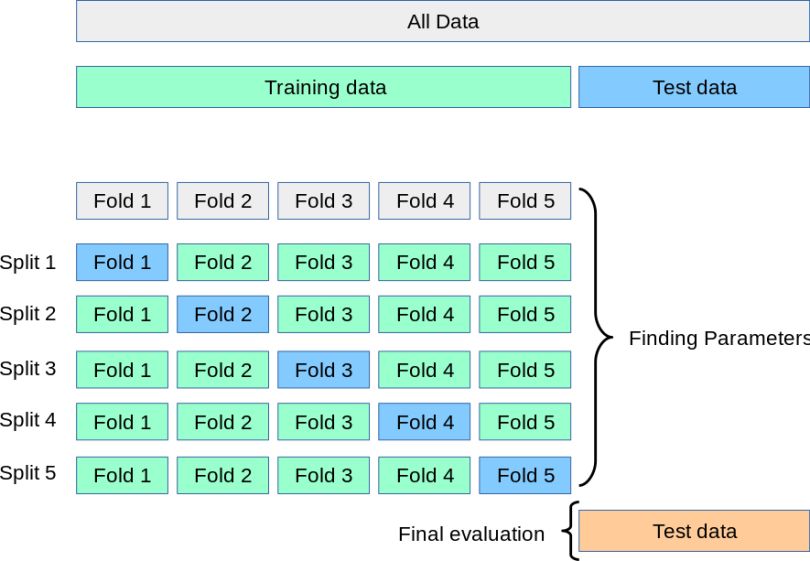
5.3.2.1. K-Fold Cross Validation
- The dataset is split into K equally sized “folds”.
- The model is trained on K−1 folds and tested on the remaining 1 fold.
- This process is repeated K times, each time using a different fold as the test set.
- The average performance over the K trials is used as the final evaluation metric.
- Where,
- $K$: Number of folds
- $\text{score}_i$: Evaluation metric (e.g., RMSE, MAE, R²) on the $i^{th}$ fold
- Advantages
- Reduces variance in performance estimation
- Uses the entire dataset for both training and testing
- More reliable for small to medium-sized datasets
- Disadvantages:
- Computationally expensive, especially for large datasets or complex models
- May not work well if data is not independently and identically distributed (i.i.d.)
5.4 Hyperparameter Tuning
- Hyperparameter tuning (also called hyperparameter optimization) is the process of searching for the best set of hyperparameters that maximizes a machine learning model’s performance on a given task.
- Unlike model parameters (which are learned from training data), hyperparameters are set before training and control the learning process itself.
- It determines how well a model learns and generalizes to new data.
- Poorly tuned hyperparameters can lead to:
- Underfitting (high bias, poor performance)
- Overfitting (high variance, poor generalization)
- Good tuning results in:
- Minimized loss
- Improved accuracy
- Robust performance
- Balanced bias-variance tradeoff
- It’s essential for real-world applications in healthcare, finance, autonomous driving, etc.
- Common hyperparamter for a Neural Network:
- Learning Rate (η): Controls step size in gradient descent.
- High → fast but unstable
- Low → stable but slow
- Epochs: Number of passes over entire training dataset
- Batch Size: Number of samples per gradient update
- Hidden Layers / Neurons: Affects capacity and depth of the network
- Activation Function: ReLU, Sigmoid, Tanh; adds non-linearity
- Momentum: Helps accelerate training by smoothing gradients
- Learning Rate Decay: Reduces learning rate over time
- Learning Rate (η): Controls step size in gradient descent.
- Objective: Minimize loss or maximize metric score
- Process:
- Choose a set of hyperparameters
- Train the model
- Evaluate performance (e.g., via cross-validation)
- Repeat until best configuration is found
- Mathematical Representation
where,
- θ : Set of hyperparameters
- $\mathcal{L}$: Loss function
- $f_{\theta}$: Model with configuration θ\thetaθ
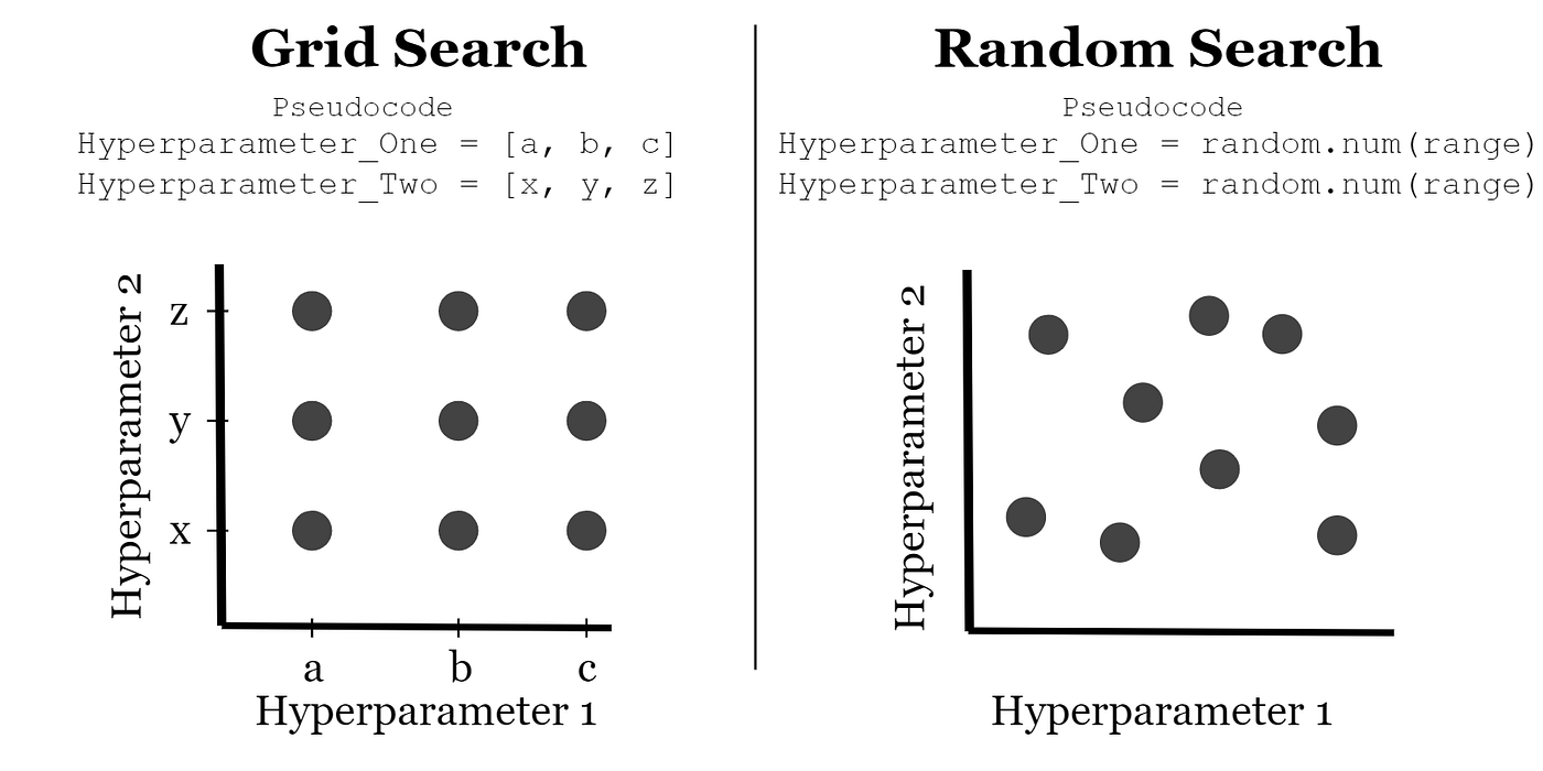
5.4.1. Grid Search
- Exhaustively tests all combinations in a hyperparameter grid
- Best for small search spaces
- Steps:
- Choose the model and its hyperparameters to tune.
- Specify a set of possible values for each hyperparameter.
- Build a grid containing all combinations.
- Train and validate the model for each combination.
- Select the combination that produces the best score (e.g., lowest MSE or highest accuracy).
- Advantages:
- Guaranteed to find optimal combo (if within grid)
- Simple to understand
- Disadvantages:
- Computationally expensive
- Doesn’t scale well with more parameters or wider ranges
- When to use:
- For small search spaces
- When computational resources are not a constraint
- When accuracy is critical and time is available
5.4.2. Random Search
- Randomly samples combinations from the search space
- Efficient when not all hyperparameters are equally important
- This process continues for a fixed number of iterations or until computational budget is exhausted.
- Advantages:
- Much faster than grid search
- Can explore larger spaces with fewer evaluations
- Disadvantages:
- No guarantee of finding the absolute best configuration
- Results may vary between runs (unless random seed is fixed)
- Might miss promising combinations if not enough iterations
- Steps:
- Select model to tune
- Define distributions for hyperparameters
- Set number of iterations (e.g., 10–100)
- Choose evaluation metric (e.g., accuracy, RMSE)
- Randomly sample hyperparameter combinations
- Train and validate model for each combination
- Compare scores across all runs
- Pick best combination
- (Optional) Retrain model on full data
- When to use:
- When hyperparameter space is large
- When computational resources or time are limited
- When exact optimal values are not critical, but good performance is sufficient